[1]:
import numpy as np
import pandas as pd
import matplotlib.pyplot as plt
from sklearn.model_selection import train_test_split
from sklearn.metrics import accuracy_score
from math import log
from copy import deepcopy

from odtlearn.datasets import robust_example
from odtlearn.robust_oct import RobustOCT
RobustOCT Examples
Example 1: Synthetic Data Without Specified Shifts
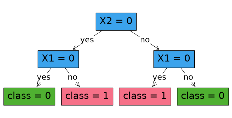
If costs and/or budget is not specified, then we will produce the same result as an optimal strong classification tree.
As an example, say that we are given this training set:
[2]:
"""
    X2
    |               |
    |               |
    1    + +        |    -
    |               |
    |---------------|-------------
    |               |
    0    - - - -    |    + + +
    |    - - -      |
    |______0________|_______1_______X1
"""
X = np.array(
    [
        [0, 0],
        [0, 0],
        [0, 0],
        [0, 0],
        [0, 0],
        [0, 0],
        [0, 0],
        [1, 0],
        [1, 0],
        [1, 0],
        [1, 1],
        [0, 1],
        [0, 1],
    ]
)
X = pd.DataFrame(X, columns=["X1", "X2"])

y = np.array([0, 0, 0, 0, 0, 0, 0, 1, 1, 1, 0, 1, 1])
If either costs or budget is not specified, the optimal classification tree will be produced (i.e., a tree that does not account for distribution shifts).
[3]:
robust_classifier = RobustOCT(
        solver="gurobi",
        depth = 2,
        time_limit = 100,
    )
robust_classifier.fit(X, y)
predictions = robust_classifier.predict(X)
Restricted license - for non-production use only - expires 2027-11-29
Set parameter TimeLimit to value 100
Set parameter LazyConstraints to value 1
Gurobi Optimizer version 13.0.2 build v13.0.2rc1 (linux64 - "Ubuntu 24.04.4 LTS")

CPU model: AMD EPYC 9V74 80-Core Processor, instruction set [SSE2|AVX|AVX2]
Thread count: 2 physical cores, 4 logical processors, using up to 4 threads

Non-default parameters:
TimeLimit  100
LazyConstraints  1

Optimize a model with 7 rows, 33 columns and 20 nonzeros (Max)
Model fingerprint: 0x78ba3dea
Model has 19 linear objective coefficients
Variable types: 13 continuous, 20 integer (20 binary)
Coefficient statistics:
  Matrix range     [1e+00, 1e+00]
  Objective range  [2e-01, 1e+00]
  Bounds range     [1e+00, 1e+00]
  RHS range        [1e+00, 1e+00]

Presolve removed 4 rows and 4 columns
Presolve time: 0.00s
Presolved: 3 rows, 29 columns, 12 nonzeros
Variable types: 13 continuous, 16 integer (16 binary)

Root relaxation: objective 1.300000e+01, 5 iterations, 0.00 seconds (0.00 work units)

    Nodes    |    Current Node    |     Objective Bounds      |     Work
 Expl Unexpl |  Obj  Depth IntInf | Incumbent    BestBd   Gap | It/Node Time

     0     0   13.00000    0    -          -   13.00000      -     -    0s
     0     0   12.75000    0    -          -   12.75000      -     -    0s
     0     0   12.75000    0    -          -   12.75000      -     -    0s
     0     0   12.50000    0    6          -   12.50000      -     -    0s
H    0     0                       7.2500000   12.50000  72.4%     -    0s
H    0     0                       9.2500000   12.50000  35.1%     -    0s
H    0     0                      10.2500000   12.50000  22.0%     -    0s
H    0     0                      12.2500000   12.50000  2.04%     -    0s
     0     0   12.50000    0    6   12.25000   12.50000  2.04%     -    0s
     0     0     cutoff    0        12.25000   12.25000  0.00%     -    0s

Cutting planes:
  Gomory: 1
  MIR: 1

Explored 1 nodes (15 simplex iterations) in 0.05 seconds (0.00 work units)
Thread count was 4 (of 4 available processors)

Solution count 4: 12.25 10.25 9.25 7.25

Optimal solution found (tolerance 1.00e-04)
Best objective 1.225000000000e+01, best bound 1.225000000000e+01, gap 0.0000%

User-callback calls 164, time in user-callback 0.03 sec
[4]:
robust_classifier.print_tree()
#########node  1
Feature:  X2 , Cutoff:  0
#########node  2
Feature:  X1 , Cutoff:  0
#########node  3
Feature:  X1 , Cutoff:  0
#########node  4
leaf 0
#########node  5
leaf 1
#########node  6
leaf 1
#########node  7
leaf 0
[5]:
fig, ax = plt.subplots(figsize=(10, 5))
robust_classifier.plot_tree()
plt.show()
Example 2: synthetic data with specified shifts
We take the same synthetic data from Example 1, but now add distribution shifts with the following schema:
For 5 samples at
![[0,0]](../_images/math/ebf9e680273a1d5e209eb0e2a4b13a19620a103b.png) , pay a cost of 1 to perturb
, pay a cost of 1 to perturb  and get
 ![[1,0]](../_images/math/89373012d8df0f30839ffc7ef5cb142d7a990cb0.png)
For the 1 sample at
![[1,1]](../_images/math/6cf1b5020649f69c2f029417055708155cca1ece.png) , pay a cost of 1 to perturb
, pay a cost of 1 to perturb  to get
 All other perturbations are not allowed
First, define these costs, which have the same shape and features as your input sample.
[6]:
# Note: 10 is a proxy for infinite cost, as it is over the allowed budgets we will specify
costs = np.array([[1,10],[1,10],[1,10],[1,10],[1,10],[10,10],[10,10],
                  [10,10],[10,10],[10,10],
                  [10,1],
                  [10,10],[10,10]])
costs = pd.DataFrame(costs, columns=['X1', 'X2'])
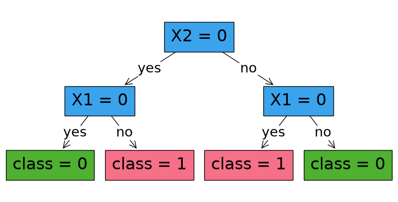
When the budget is 2 (corresponding to the variable ε), we don’t see a change in the tree from Example 1 since for this dataset, the budget is small and thus the level of robustness is small.
[7]:
# Same data as Example 1
X = np.array(
    [
        [0, 0],
        [0, 0],
        [0, 0],
        [0, 0],
        [0, 0],
        [0, 0],
        [0, 0],
        [1, 0],
        [1, 0],
        [1, 0],
        [1, 1],
        [0, 1],
        [0, 1],
    ]
)
X = pd.DataFrame(X, columns=["X1", "X2"])

y = np.array([0, 0, 0, 0, 0, 0, 0, 1, 1, 1, 0, 1, 1])
[8]:
robust_classifier = RobustOCT(
    solver="gurobi",
    depth=2,
    time_limit=100
)
robust_classifier.fit(X, y, costs=costs, budget=2)
predictions = robust_classifier.predict(X)
Set parameter TimeLimit to value 100
Set parameter LazyConstraints to value 1
Gurobi Optimizer version 13.0.2 build v13.0.2rc1 (linux64 - "Ubuntu 24.04.4 LTS")

CPU model: AMD EPYC 9V74 80-Core Processor, instruction set [SSE2|AVX|AVX2]
Thread count: 2 physical cores, 4 logical processors, using up to 4 threads

Non-default parameters:
TimeLimit  100
LazyConstraints  1

Optimize a model with 7 rows, 33 columns and 20 nonzeros (Max)
Model fingerprint: 0x78ba3dea
Model has 19 linear objective coefficients
Variable types: 13 continuous, 20 integer (20 binary)
Coefficient statistics:
  Matrix range     [1e+00, 1e+00]
  Objective range  [2e-01, 1e+00]
  Bounds range     [1e+00, 1e+00]
  RHS range        [1e+00, 1e+00]

Presolve removed 4 rows and 4 columns
Presolve time: 0.00s
Presolved: 3 rows, 29 columns, 12 nonzeros
Variable types: 13 continuous, 16 integer (16 binary)

Root relaxation: objective 1.300000e+01, 5 iterations, 0.00 seconds (0.00 work units)

    Nodes    |    Current Node    |     Objective Bounds      |     Work
 Expl Unexpl |  Obj  Depth IntInf | Incumbent    BestBd   Gap | It/Node Time

     0     0   13.00000    0    -          -   13.00000      -     -    0s
     0     0   12.75000    0    -          -   12.75000      -     -    0s
     0     0   12.75000    0    -          -   12.75000      -     -    0s
     0     0   12.50000    0    6          -   12.50000      -     -    0s
H    0     0                       7.2500000   12.50000  72.4%     -    0s
H    0     0                       9.2500000   12.50000  35.1%     -    0s
H    0     0                      10.2500000   12.50000  22.0%     -    0s
     0     0   12.50000    0    6   10.25000   12.50000  22.0%     -    0s
     0     0   12.25000    0    -   10.25000   12.25000  19.5%     -    0s
     0     0   12.25000    0    6   10.25000   12.25000  19.5%     -    0s
     0     0   12.22477    0    8   10.25000   12.22477  19.3%     -    0s
     0     0   12.18964    0    8   10.25000   12.18964  18.9%     -    0s
     0     0   12.18964    0    8   10.25000   12.18964  18.9%     -    0s
     0     0   12.18964    0    8   10.25000   12.18964  18.9%     -    0s
     0     0   12.18964    0    8   10.25000   12.18964  18.9%     -    0s
     0     0   12.18964    0    8   10.25000   12.18964  18.9%     -    0s
     0     2   12.18964    0    8   10.25000   12.18964  18.9%     -    0s

Cutting planes:
  Gomory: 1
  MIR: 1
  RLT: 2

Explored 45 nodes (215 simplex iterations) in 0.08 seconds (0.01 work units)
Thread count was 4 (of 4 available processors)

Solution count 3: 10.25 9.25 7.25

Optimal solution found (tolerance 1.00e-04)
Best objective 1.025000000000e+01, best bound 1.025000000000e+01, gap 0.0000%

User-callback calls 294, time in user-callback 0.05 sec
[9]:
robust_classifier.print_tree()
#########node  1
Feature:  X2 , Cutoff:  0
#########node  2
Feature:  X1 , Cutoff:  0
#########node  3
Feature:  X1 , Cutoff:  0
#########node  4
leaf 0
#########node  5
leaf 1
#########node  6
leaf 1
#########node  7
leaf 0
[10]:
fig, ax = plt.subplots(figsize=(10, 5))
robust_classifier.plot_tree()
plt.show()
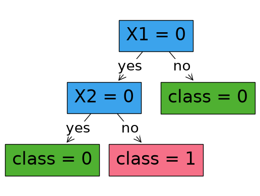
But when the budget is increased to 5 (adding more robustness), we see a change in the tree.
[11]:
robust_classifier = RobustOCT(
    solver="gurobi",
    depth=2,
    time_limit=100
)
robust_classifier.fit(X, y, costs=costs, budget=5)
predictions = robust_classifier.predict(X)
Set parameter TimeLimit to value 100
Set parameter LazyConstraints to value 1
Gurobi Optimizer version 13.0.2 build v13.0.2rc1 (linux64 - "Ubuntu 24.04.4 LTS")

CPU model: AMD EPYC 9V74 80-Core Processor, instruction set [SSE2|AVX|AVX2]
Thread count: 2 physical cores, 4 logical processors, using up to 4 threads

Non-default parameters:
TimeLimit  100
LazyConstraints  1

Optimize a model with 7 rows, 33 columns and 20 nonzeros (Max)
Model fingerprint: 0x78ba3dea
Model has 19 linear objective coefficients
Variable types: 13 continuous, 20 integer (20 binary)
Coefficient statistics:
  Matrix range     [1e+00, 1e+00]
  Objective range  [2e-01, 1e+00]
  Bounds range     [1e+00, 1e+00]
  RHS range        [1e+00, 1e+00]

Presolve removed 4 rows and 4 columns
Presolve time: 0.00s
Presolved: 3 rows, 29 columns, 12 nonzeros
Variable types: 13 continuous, 16 integer (16 binary)

Root relaxation: objective 1.300000e+01, 5 iterations, 0.00 seconds (0.00 work units)

    Nodes    |    Current Node    |     Objective Bounds      |     Work
 Expl Unexpl |  Obj  Depth IntInf | Incumbent    BestBd   Gap | It/Node Time

     0     0   13.00000    0    -          -   13.00000      -     -    0s
     0     0   12.75000    0    -          -   12.75000      -     -    0s
     0     0   12.75000    0    -          -   12.75000      -     -    0s
     0     0   12.50000    0    6          -   12.50000      -     -    0s
H    0     0                       7.2500000   12.50000  72.4%     -    0s
H    0     0                       9.2500000   12.50000  35.1%     -    0s
     0     0   12.50000    0    6    9.25000   12.50000  35.1%     -    0s
     0     0   12.25000    0    -    9.25000   12.25000  32.4%     -    0s
     0     0   12.25000    0    6    9.25000   12.25000  32.4%     -    0s
     0     0   12.25000    0    6    9.25000   12.25000  32.4%     -    0s
     0     0   12.25000    0    6    9.25000   12.25000  32.4%     -    0s
     0     2   12.25000    0    6    9.25000   12.25000  32.4%     -    0s
*   48     0               5       9.5000000   10.43333  9.82%   4.5    0s

Cutting planes:
  Gomory: 1
  MIR: 1

Explored 54 nodes (266 simplex iterations) in 0.16 seconds (0.00 work units)
Thread count was 4 (of 4 available processors)

Solution count 3: 9.5 9.25 7.25

Optimal solution found (tolerance 1.00e-04)
Best objective 9.500000000000e+00, best bound 9.500000000000e+00, gap 0.0000%

User-callback calls 298, time in user-callback 0.13 sec
[12]:
robust_classifier.print_tree()
#########node  1
Feature:  X1 , Cutoff:  0
#########node  2
Feature:  X2 , Cutoff:  0
#########node  3
leaf 0
#########node  4
leaf 0
#########node  5
leaf 1
#########node  6
pruned
#########node  7
pruned
[13]:
robust_classifier.plot_tree()
plt.show()
Example 3: UCI data example
Here, we’ll see the benefits of using robust optimization by perturbing the test set. We will use the MONK’s Problems dataset from the UCI Machine Learning Repository.
Fetch data and split to train and test
[14]:
"""Fetch data and split to train and test"""
data, y = robust_example()

X_train, X_test, y_train, y_test = train_test_split(
    data, y, test_size=0.25, random_state=2
)
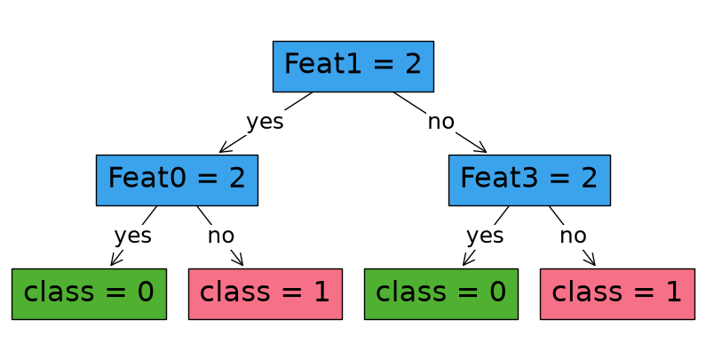
For sake of comparison, train a classification tree that does not consider the scenario where there is a distribution shift:
[15]:
"""Train a non-robust tree for comparison"""

# If you define no uncertainty, you get an optimal tree without regularization that maximizes accuracy
non_robust_classifier = RobustOCT(solver="gurobi", depth=2, time_limit=300)
non_robust_classifier.fit(X_train, y_train)
Set parameter TimeLimit to value 300
Set parameter LazyConstraints to value 1
Gurobi Optimizer version 13.0.2 build v13.0.2rc1 (linux64 - "Ubuntu 24.04.4 LTS")

CPU model: AMD EPYC 9V74 80-Core Processor, instruction set [SSE2|AVX|AVX2]
Thread count: 2 physical cores, 4 logical processors, using up to 4 threads

Non-default parameters:
TimeLimit  300
LazyConstraints  1

Optimize a model with 7 rows, 173 columns and 47 nonzeros (Max)
Model fingerprint: 0xafd32360
Model has 159 linear objective coefficients
Variable types: 126 continuous, 47 integer (47 binary)
Coefficient statistics:
  Matrix range     [1e+00, 1e+00]
  Objective range  [2e-01, 1e+00]
  Bounds range     [1e+00, 1e+00]
  RHS range        [1e+00, 1e+00]

Presolve removed 4 rows and 4 columns
Presolve time: 0.00s
Presolved: 3 rows, 169 columns, 39 nonzeros
Variable types: 126 continuous, 43 integer (43 binary)

Root relaxation: objective 1.260000e+02, 5 iterations, 0.00 seconds (0.00 work units)

    Nodes    |    Current Node    |     Objective Bounds      |     Work
 Expl Unexpl |  Obj  Depth IntInf | Incumbent    BestBd   Gap | It/Node Time

     0     0  126.00000    0    -          -  126.00000      -     -    0s
     0     0  125.75000    0    -          -  125.75000      -     -    0s
     0     0  125.75000    0    7          -  125.75000      -     -    0s
H    0     0                      77.2500000  125.75000  62.8%     -    0s
H    0     0                      78.0000000  125.75000  61.2%     -    0s
     0     0  125.55000    0   13   78.00000  125.55000  61.0%     -    0s
     0     0  125.43182    0   18   78.00000  125.43182  60.8%     -    0s
     0     0  125.31818    0   22   78.00000  125.31818  60.7%     -    0s
     0     0  125.29167    0   22   78.00000  125.29167  60.6%     -    0s
     0     0  125.29167    0   22   78.00000  125.29167  60.6%     -    0s
     0     2  125.29167    0   22   78.00000  125.29167  60.6%     -    0s
*  283   205              18      78.2500000  122.25000  56.2%  25.9    1s
H  344   244                      80.2500000  122.25000  52.3%  27.2    1s
*  351   241              27      80.5000000  122.25000  51.9%  26.9    2s
*  489   297              21      81.2500000  118.83333  46.3%  25.2    2s
*  513   310              23      81.5000000  118.82895  45.8%  25.0    2s
*  692   358              15      82.2500000  114.87500  39.7%  24.7    2s
*  819   368              16      82.5000000  112.95000  36.9%  25.1    2s
* 1182   461              15      83.2500000  105.94444  27.3%  22.7    2s

Cutting planes:
  Gomory: 3
  MIR: 1
  Flow cover: 39
  RLT: 1

Explored 5449 nodes (101910 simplex iterations) in 4.85 seconds (4.02 work units)
Thread count was 4 (of 4 available processors)

Solution count 10: 83.25 82.5 82.25 ... 77.25

Optimal solution found (tolerance 1.00e-04)
Best objective 8.325000000000e+01, best bound 8.325000000000e+01, gap 0.0000%

User-callback calls 11562, time in user-callback 2.24 sec
[15]:
RobustOCT(solver=gurobi,depth=2,time_limit=300,num_threads=None,verbose=False)
[16]:
non_robust_classifier.print_tree()
#########node  1
Feature:  Feat1 , Cutoff:  2
#########node  2
Feature:  Feat0 , Cutoff:  2
#########node  3
Feature:  Feat3 , Cutoff:  2
#########node  4
leaf 0
#########node  5
leaf 1
#########node  6
leaf 0
#########node  7
leaf 1
[17]:
fig, ax = plt.subplots(figsize=(10, 5))
non_robust_classifier.plot_tree()
plt.show()
Train a robust tree. First, define the uncertainty. Here, we will generate a probability of certainty for each feature randomly (in practice, you would need to use some guess from domain knowledge). For simplicity, we will not change this probability by data sample  . We also define
  , which in practice must be tuned.
[18]:
"""Generate q_f values for each feature (i.e. probability of certainty for feature f)"""
np.random.seed(42)
q_f = np.random.normal(loc=0.9, scale=0.1, size=len(X_train.columns))
# Snap q_f to range [0,1]
q_f[q_f <= 0] = np.nextafter(np.float32(0), np.float32(1))
q_f[q_f > 1] = 1.0

q_f
[18]:
array([0.94967142, 0.88617357, 0.96476885, 1.        , 0.87658466,
       0.8765863 ])
Calibrate the costs and budget parameters for the fit function.
[19]:
"""Define budget of uncertainty"""

l = 0.9  # Lambda value between 0 and 1
budget = -1 * X_train.shape[0] * log(l)
budget
[19]:
13.275424972886112
[20]:
"""Based on q_f values, create costs of uncertainty"""
costs = deepcopy(X_train)
costs = costs.astype("float")
for f in range(len(q_f)):
    if q_f[f] == 1:
        costs[costs.columns[f]] = budget + 1  # no uncertainty = "infinite" cost
    else:
        costs[costs.columns[f]] = -1 * log(1 - q_f[f])

costs
[20]:
| Feat0 | Feat1 | Feat2 | Feat3 | Feat4 | Feat5 | |
|---|---|---|---|---|---|---|
| 0 | 2.989182 | 2.173081 | 3.345825 | 14.275425 | 2.0922 | 2.092213 |
| 1 | 2.989182 | 2.173081 | 3.345825 | 14.275425 | 2.0922 | 2.092213 |
| 2 | 2.989182 | 2.173081 | 3.345825 | 14.275425 | 2.0922 | 2.092213 |
| 3 | 2.989182 | 2.173081 | 3.345825 | 14.275425 | 2.0922 | 2.092213 |
| 4 | 2.989182 | 2.173081 | 3.345825 | 14.275425 | 2.0922 | 2.092213 |
| ... | ... | ... | ... | ... | ... | ... |
| 121 | 2.989182 | 2.173081 | 3.345825 | 14.275425 | 2.0922 | 2.092213 |
| 122 | 2.989182 | 2.173081 | 3.345825 | 14.275425 | 2.0922 | 2.092213 |
| 123 | 2.989182 | 2.173081 | 3.345825 | 14.275425 | 2.0922 | 2.092213 |
| 124 | 2.989182 | 2.173081 | 3.345825 | 14.275425 | 2.0922 | 2.092213 |
| 125 | 2.989182 | 2.173081 | 3.345825 | 14.275425 | 2.0922 | 2.092213 |
126 rows × 6 columns
Train the robust tree using the costs and budget.
[21]:
robust_classifier = RobustOCT(
    solver="gurobi",
    depth=2,
    time_limit=200,
)
robust_classifier.fit(X_train, y_train, costs=costs, budget=budget)
Set parameter TimeLimit to value 200
Set parameter LazyConstraints to value 1
Gurobi Optimizer version 13.0.2 build v13.0.2rc1 (linux64 - "Ubuntu 24.04.4 LTS")

CPU model: AMD EPYC 9V74 80-Core Processor, instruction set [SSE2|AVX|AVX2]
Thread count: 2 physical cores, 4 logical processors, using up to 4 threads

Non-default parameters:
TimeLimit  200
LazyConstraints  1

Optimize a model with 7 rows, 173 columns and 47 nonzeros (Max)
Model fingerprint: 0xafd32360
Model has 159 linear objective coefficients
Variable types: 126 continuous, 47 integer (47 binary)
Coefficient statistics:
  Matrix range     [1e+00, 1e+00]
  Objective range  [2e-01, 1e+00]
  Bounds range     [1e+00, 1e+00]
  RHS range        [1e+00, 1e+00]

Presolve removed 4 rows and 4 columns
Presolve time: 0.00s
Presolved: 3 rows, 169 columns, 39 nonzeros
Variable types: 126 continuous, 43 integer (43 binary)

Root relaxation: objective 1.260000e+02, 5 iterations, 0.00 seconds (0.00 work units)

    Nodes    |    Current Node    |     Objective Bounds      |     Work
 Expl Unexpl |  Obj  Depth IntInf | Incumbent    BestBd   Gap | It/Node Time

     0     0  126.00000    0    -          -  126.00000      -     -    0s
     0     0  125.75000    0    -          -  125.75000      -     -    0s
     0     0  125.75000    0    7          -  125.75000      -     -    0s
H    0     0                      77.2500000  125.75000  62.8%     -    0s
H    0     0                      78.0000000  125.75000  61.2%     -    0s
     0     0  125.55000    0   13   78.00000  125.55000  61.0%     -    0s
     0     0  125.43182    0   18   78.00000  125.43182  60.8%     -    0s
     0     0  125.31818    0   22   78.00000  125.31818  60.7%     -    0s
     0     0  125.29167    0   22   78.00000  125.29167  60.6%     -    0s
     0     0  125.29167    0   20   78.00000  125.29167  60.6%     -    0s
     0     2  125.29167    0   20   78.00000  125.29167  60.6%     -    0s
   975   621   85.58333   12    5   78.00000  112.69697  44.5%  24.3    5s
H 1499   721                      78.5000000  110.37500  40.6%  25.3    8s
H 1812   720                      79.5000000  110.37500  38.8%  24.7    9s
  1937   740   92.08333   26    5   79.50000  110.37500  38.8%  24.1   10s
  3807   957   85.50000   38    2   79.50000   95.25000  19.8%  17.5   15s
  5065   740   80.00000   32    4   79.50000   88.90000  11.8%  15.9   20s
  6395   186   81.12500   27    2   79.50000   81.75000  2.83%  14.6   25s

Cutting planes:
  MIR: 2
  Flow cover: 54
  RLT: 1

Explored 6743 nodes (95373 simplex iterations) in 26.87 seconds (7.34 work units)
Thread count was 4 (of 4 available processors)

Solution count 5: 79.5 78.5 78 ... 77.25

Optimal solution found (tolerance 1.00e-04)
Best objective 7.950000000000e+01, best bound 7.950000000000e+01, gap 0.0000%

User-callback calls 14865, time in user-callback 22.13 sec
[21]:
RobustOCT(solver=gurobi,depth=2,time_limit=200,num_threads=None,verbose=False)
[22]:
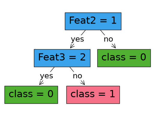
robust_classifier.print_tree()
#########node  1
Feature:  Feat2 , Cutoff:  1
#########node  2
Feature:  Feat3 , Cutoff:  2
#########node  3
leaf 0
#########node  4
leaf 0
#########node  5
leaf 1
#########node  6
pruned
#########node  7
pruned
[23]:
robust_classifier.plot_tree()
plt.show()
[24]:
print(
    "Non-robust training accuracy: ",
    accuracy_score(y_train, non_robust_classifier.predict(X_train)),
)
print(
    "Robust training accuracy:     ",
    accuracy_score(y_train, robust_classifier.predict(X_train)),
)
print(
    "Non-robust test accuracy:     ",
    accuracy_score(y_test, non_robust_classifier.predict(X_test)),
)
print(
    "Robust test accuracy:         ",
    accuracy_score(y_test, robust_classifier.predict(X_test)),
)
Non-robust training accuracy:  0.6666666666666666
Robust training accuracy:      0.6587301587301587
Non-robust test accuracy:      0.46511627906976744
Robust test accuracy:          0.5581395348837209
To measure the performance of the trained models, perturb the test data based off of our known certainties of each feature (to simulate a distribtion shift), and then see how well each tree performs against the perturbed data
[25]:
def perturb(data, q_f, seed):
    """Perturb X given q_f based off of the symmetric geometric distribution"""
    new_data = deepcopy(data)
    np.random.seed(seed)
    # Perturbation of features
    for f in range(len(new_data.columns)):
        perturbations = np.random.geometric(q_f[f], size=new_data.shape[0])
        perturbations = perturbations - 1  # Support should be 0,1,2,...
        signs = (2 * np.random.binomial(1, 0.5, size=new_data.shape[0])) - 1
        perturbations = perturbations * signs
        new_data[new_data.columns[f]] = new_data[new_data.columns[f]] + perturbations
    return new_data


"""Obtain 1000 different perturbed test sets, and record accuracies"""
non_robust_acc = []
robust_acc = []
for s in range(1, 1001):
    X_test_perturbed = perturb(X_test, q_f, s)
    non_robust_pred = non_robust_classifier.predict(X_test_perturbed)
    robust_pred = robust_classifier.predict(X_test_perturbed)
    non_robust_acc += [accuracy_score(y_test, non_robust_pred)]
    robust_acc += [accuracy_score(y_test, robust_pred)]
[26]:
print("Worst-case accuracy (Non-Robust Tree): ", min(non_robust_acc))
print("Worst-case accuracy (Robust Tree):     ", min(robust_acc))
print(
    "Average accuracy (Non-Robust Tree):    ", sum(non_robust_acc) / len(non_robust_acc)
)
print("Average accuracy (Robust Tree):        ", sum(robust_acc) / len(robust_acc))
Worst-case accuracy (Non-Robust Tree):  0.3953488372093023
Worst-case accuracy (Robust Tree):      0.5116279069767442
Average accuracy (Non-Robust Tree):     0.47367441860465515
Average accuracy (Robust Tree):         0.5584186046511533
References
Justin, N., Aghaei, S., Gómez, A., & Vayanos, P. (2021). Optimal robust classification trees. The AAAI-2022 Workshop on Adversarial Machine Learning and Beyond. https://openreview.net/pdf?id=HbasA9ysA3
Justin, N., Aghaei, S., Gómez, A., & Vayanos, P. (2023). Learning optimal classification trees robust to distribution shifts. arXiv preprint arXiv:2310.17772.
Dua, D. and Graff, C. (2019). UCI Machine Learning Repository. Irvine, CA: University of California, School of Information and Computer Science.
[ ]: