[1]:
import numpy as np
import pandas as pd
import matplotlib.pyplot as plt

from odtlearn.flow_oct import FlowOCT, BendersOCT
from odtlearn.utils.binarize import Binarizer
FlowOCT Examples
Example 0: Binarization
The following example shows how to binarize a dataset with categorical, integer, and continuous features using the built-in Binarizer class. This class follows the scikit-learn fit-transform paradigm, making it easy to integrate into your preprocessing pipeline.
[2]:
number_of_child_list = [1, 2, 4, 3, 1, 2, 4, 3, 2, 1]
age_list = [10, 20, 40, 30, 10, 20, 40, 30, 20, 10]
race_list = [
    "Black",
    "White",
    "Hispanic",
    "Black",
    "White",
    "Black",
    "White",
    "Hispanic",
    "Black",
    "White",
]
sex_list = ["M", "F", "M", "M", "F", "M", "F", "M", "M", "F"]
income_list = [50000, 75000, 100000, 60000, 80000, 55000, 90000, 70000, 85000, 65000]

df = pd.DataFrame(
    list(zip(sex_list, race_list, number_of_child_list, age_list, income_list)),
    columns=["sex", "race", "num_child", "age", "income"],
)

print(df)
  sex      race  num_child  age  income
0   M     Black          1   10   50000
1   F     White          2   20   75000
2   M  Hispanic          4   40  100000
3   M     Black          3   30   60000
4   F     White          1   10   80000
5   M     Black          2   20   55000
6   F     White          4   40   90000
7   M  Hispanic          3   30   70000
8   M     Black          2   20   85000
9   F     White          1   10   65000
[3]:
binarizer = Binarizer(
    categorical_cols=["sex", "race"],
    integer_cols=["num_child", "age"],
    real_cols=["income"],
    n_bins=5  # Number of bins for continuous features
)

# Fit and transform the data
df_enc = binarizer.fit_transform(df)

print(df_enc)
   sex_M  race_Black  race_Hispanic  race_White  num_child_1  num_child_2  \
0    1.0         1.0            0.0         0.0          1.0          1.0
1    0.0         0.0            0.0         1.0          0.0          1.0
2    1.0         0.0            1.0         0.0          0.0          0.0
3    1.0         1.0            0.0         0.0          0.0          0.0
4    0.0         0.0            0.0         1.0          1.0          1.0
5    1.0         1.0            0.0         0.0          0.0          1.0
6    0.0         0.0            0.0         1.0          0.0          0.0
7    1.0         0.0            1.0         0.0          0.0          0.0
8    1.0         1.0            0.0         0.0          0.0          1.0
9    0.0         0.0            0.0         1.0          1.0          1.0

   num_child_3  num_child_4  age_10  age_20  age_30  age_40  income_0  \
0          1.0          1.0     1.0     1.0     1.0     1.0       1.0
1          1.0          1.0     0.0     1.0     1.0     1.0       0.0
2          0.0          1.0     0.0     0.0     0.0     1.0       0.0
3          1.0          1.0     0.0     0.0     1.0     1.0       0.0
4          1.0          1.0     1.0     1.0     1.0     1.0       0.0
5          1.0          1.0     0.0     1.0     1.0     1.0       1.0
6          0.0          1.0     0.0     0.0     0.0     1.0       0.0
7          1.0          1.0     0.0     0.0     1.0     1.0       0.0
8          1.0          1.0     0.0     1.0     1.0     1.0       0.0
9          1.0          1.0     1.0     1.0     1.0     1.0       0.0

   income_1  income_2  income_3  income_4
0       1.0       1.0       1.0       1.0
1       0.0       1.0       1.0       1.0
2       0.0       0.0       0.0       1.0
3       1.0       1.0       1.0       1.0
4       0.0       0.0       1.0       1.0
5       1.0       1.0       1.0       1.0
6       0.0       0.0       0.0       1.0
7       0.0       1.0       1.0       1.0
8       0.0       0.0       1.0       1.0
9       1.0       1.0       1.0       1.0
The Binarizer class follows the scikit-learn fit-transform paradigm:
We initialize the Binarizer with our desired parameters, specifying which columns are categorical, integer, and real-valued. We call the fit_transform method, which first fits the binarizer to our data (learning the necessary encoding schemes) and then transforms the data using those learned encodings.
The resulting df_enc DataFrame contains the binarized version of our original data:
Categorical columns (sex, race) are one-hot encoded. Integer columns (num_child, age) are binary encoded, where each column represents “greater than or equal to” a certain value. The continuous column (income) is first discretized into 5 bins, then binary encoded similar to the integer columns.
[4]:
print(df_enc.columns)
Index(['sex_M', 'race_Black', 'race_Hispanic', 'race_White', 'num_child_1',
       'num_child_2', 'num_child_3', 'num_child_4', 'age_10', 'age_20',
       'age_30', 'age_40', 'income_0', 'income_1', 'income_2', 'income_3',
       'income_4'],
      dtype='object')
This binarized data is now ready to be used with any of the models in ODTlearn, which require binary input features. If you need to transform new data using the same encoding scheme, you can use the transform method of the fitted binarizer:
[5]:
new_data = pd.DataFrame({
    "sex": ["F", "M"],
    "race": ["Hispanic", "White"],
    "num_child": [2, 3],
    "age": [20, 30],
    "income": [70000, 80000]
})

new_data_enc = binarizer.transform(new_data)
print(new_data_enc)
   sex_M  race_Black  race_Hispanic  race_White  num_child_1  num_child_2  \
0    0.0         0.0            1.0         0.0          0.0          1.0
1    1.0         0.0            0.0         1.0          0.0          0.0

   num_child_3  num_child_4  age_10  age_20  age_30  age_40  income_0  \
0          1.0          1.0     0.0     1.0     1.0     1.0         0
1          1.0          1.0     0.0     0.0     1.0     1.0         0

   income_1  income_2  income_3  income_4
0         0       1.0       1.0         0
1         0       0.0       1.0         0
Note that for categorical features, if the new data contains categories not seen during fitting, the transform method will raise an error. In such cases, you might need to refit the binarizer on a dataset that includes all possible categories.
Example 1: Varying depth and _lambda
In this part, we study a simple example and investigate different parameter combinations to provide intuition on how they affect the structure of the tree.
First we generate the data for our example. The diagram within the code block shows the training dataset. Our dataset has two binary features (X1 and X2) and two class labels (+1 and -1).
[6]:
from odtlearn.datasets import flow_oct_example

"""
    X2
    |               |
    |               |
    1    + +        |    -
    |               |
    |---------------|-------------
    |               |
    0    - - - -    |    + + +
    |    - - -      |
    |______0________|_______1_______X1
"""


X, y = flow_oct_example()
Tree with depth = 1
In the following, we fit a classification tree of depth 1, i.e., a tree with a single branching node and two leaf nodes.
[7]:
stcl = FlowOCT(depth=1, solver="gurobi", time_limit=100)
stcl.store_search_progress_log = True
stcl.fit(X, y)
Set parameter Username
Academic license - for non-commercial use only - expires 2025-06-28
Set parameter TimeLimit to value 100
Set parameter NodeLimit to value 1073741824
Set parameter SolutionLimit to value 1073741824
Set parameter IntFeasTol to value 1e-06
Set parameter Method to value 3
Gurobi Optimizer version 10.0.2 build v10.0.2rc0 (mac64[arm])

CPU model: Apple M1 Pro
Thread count: 8 physical cores, 8 logical processors, using up to 8 threads

Optimize a model with 110 rows, 89 columns and 250 nonzeros
Model fingerprint: 0x5e9209d1
Variable types: 84 continuous, 5 integer (5 binary)
Coefficient statistics:
  Matrix range     [1e+00, 1e+00]
  Objective range  [1e+00, 1e+00]
  Bounds range     [1e+00, 1e+00]
  RHS range        [1e+00, 1e+00]
Presolve removed 102 rows and 82 columns
Presolve time: 0.00s
Presolved: 8 rows, 7 columns, 16 nonzeros
Variable types: 6 continuous, 1 integer (1 binary)
Found heuristic solution: objective 9.0000000

Root relaxation: objective 1.000000e+01, 2 iterations, 0.00 seconds (0.00 work units)

    Nodes    |    Current Node    |     Objective Bounds      |     Work
 Expl Unexpl |  Obj  Depth IntInf | Incumbent    BestBd   Gap | It/Node Time

*    0     0               0      10.0000000   10.00000  0.00%     -    0s

Explored 1 nodes (2 simplex iterations) in 0.00 seconds (0.00 work units)
Thread count was 8 (of 8 available processors)

Solution count 2: 10 9

Optimal solution found (tolerance 1.00e-04)
Best objective 1.000000000000e+01, best bound 1.000000000000e+01, gap 0.0000%

User-callback calls 573, time in user-callback 0.00 sec
[7]:
FlowOCT(solver=gurobi,depth=1,time_limit=100,num_threads=None,verbose=False)
[8]:
predictions = stcl.predict(X)
print(f'Optimality gap is {stcl.optim_gap}')
print(f"In-sample accuracy is {np.sum(predictions==y)/y.shape[0]}")
Optimality gap is 0.0
In-sample accuracy is 0.7692307692307693
Users can access statistics from the optimization run such as optimality gap, number of nodes, number of constraints, etc. Directly as properties of the initialized class or through the _solver object. For example, one can access the optimality gap and the number of solutions after fitting the optimal decision tree through the optim_gap and num_solutions properties.
[9]:
print(f'Optimality gap is {stcl.optim_gap}')
print(f'Number of solutions {stcl.num_solutions}')
Optimality gap is 0.0
Number of solutions 2
As we can see above, we find the optimal tree and the in-sample accuracy is 76%.
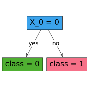
ODTlearn provides two different ways of visualizing the structure of the tree. The first method prints the structure of the tree in the console:
[10]:
stcl.print_tree()
#########node  1
branch on X_0
#########node  2
leaf 0
#########node  3
leaf 1
The second method plots the structure of the tree using matplotlib:
[11]:
fig, ax = plt.subplots(figsize=(5, 5))
stcl.plot_tree(ax=ax)
plt.show()
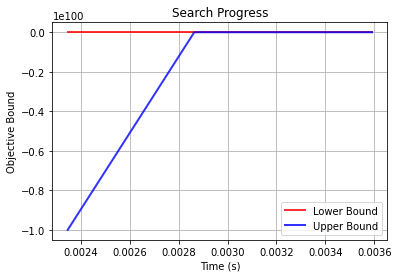
We also provide a simple function allowing users to plot the search progress log over time. Note that you must set the attribute store_search_progress_log to True before calling the fit method to ensure that the bound information is stored.
[12]:
stcl_progress_log = FlowOCT(depth=1, solver="gurobi", time_limit=100)
stcl_progress_log.store_search_progress_log = True
stcl_progress_log.fit(X, y)
Set parameter Username
Academic license - for non-commercial use only - expires 2025-06-28
Set parameter TimeLimit to value 100
Set parameter NodeLimit to value 1073741824
Set parameter SolutionLimit to value 1073741824
Set parameter IntFeasTol to value 1e-06
Set parameter Method to value 3
Gurobi Optimizer version 10.0.2 build v10.0.2rc0 (mac64[arm])

CPU model: Apple M1 Pro
Thread count: 8 physical cores, 8 logical processors, using up to 8 threads

Optimize a model with 110 rows, 89 columns and 250 nonzeros
Model fingerprint: 0x5e9209d1
Variable types: 84 continuous, 5 integer (5 binary)
Coefficient statistics:
  Matrix range     [1e+00, 1e+00]
  Objective range  [1e+00, 1e+00]
  Bounds range     [1e+00, 1e+00]
  RHS range        [1e+00, 1e+00]
Presolve removed 102 rows and 82 columns
Presolve time: 0.00s
Presolved: 8 rows, 7 columns, 16 nonzeros
Variable types: 6 continuous, 1 integer (1 binary)
Found heuristic solution: objective 9.0000000

Root relaxation: objective 1.000000e+01, 2 iterations, 0.00 seconds (0.00 work units)

    Nodes    |    Current Node    |     Objective Bounds      |     Work
 Expl Unexpl |  Obj  Depth IntInf | Incumbent    BestBd   Gap | It/Node Time

*    0     0               0      10.0000000   10.00000  0.00%     -    0s

Explored 1 nodes (2 simplex iterations) in 0.01 seconds (0.00 work units)
Thread count was 8 (of 8 available processors)

Solution count 2: 10 9

Optimal solution found (tolerance 1.00e-04)
Best objective 1.000000000000e+01, best bound 1.000000000000e+01, gap 0.0000%

User-callback calls 573, time in user-callback 0.00 sec
[12]:
FlowOCT(solver=gurobi,depth=1,time_limit=100,num_threads=None,verbose=False)
[13]:
stcl.plot_search_progress()
[13]:
<AxesSubplot:title={'center':'Search Progress'}, xlabel='Time (s)', ylabel='Objective Bound'>
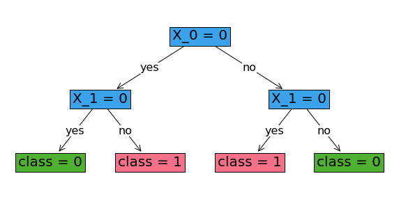
Tree with depth = 2
Now we increase the depth of the tree to achieve higher accuracy.
[14]:
stcl = FlowOCT(depth=2, solver="gurobi")
stcl.fit(X, y)
Set parameter Username
Academic license - for non-commercial use only - expires 2025-06-28
Set parameter TimeLimit to value 60
Set parameter NodeLimit to value 1073741824
Set parameter SolutionLimit to value 1073741824
Set parameter IntFeasTol to value 1e-06
Set parameter Method to value 3
Gurobi Optimizer version 10.0.2 build v10.0.2rc0 (mac64[arm])

CPU model: Apple M1 Pro
Thread count: 8 physical cores, 8 logical processors, using up to 8 threads

Optimize a model with 274 rows, 209 columns and 642 nonzeros
Model fingerprint: 0x51470803
Variable types: 196 continuous, 13 integer (13 binary)
Coefficient statistics:
  Matrix range     [1e+00, 1e+00]
  Objective range  [1e+00, 1e+00]
  Bounds range     [1e+00, 1e+00]
  RHS range        [1e+00, 1e+00]
Found heuristic solution: objective -0.0000000
Presolve removed 250 rows and 187 columns
Presolve time: 0.00s
Presolved: 24 rows, 22 columns, 76 nonzeros
Found heuristic solution: objective 8.0000000
Variable types: 16 continuous, 6 integer (6 binary)

Root relaxation: objective 1.300000e+01, 14 iterations, 0.00 seconds (0.00 work units)

    Nodes    |    Current Node    |     Objective Bounds      |     Work
 Expl Unexpl |  Obj  Depth IntInf | Incumbent    BestBd   Gap | It/Node Time

*    0     0               0      13.0000000   13.00000  0.00%     -    0s

Explored 1 nodes (14 simplex iterations) in 0.00 seconds (0.00 work units)
Thread count was 8 (of 8 available processors)

Solution count 3: 13 8 -0

Optimal solution found (tolerance 1.00e-04)
Best objective 1.300000000000e+01, best bound 1.300000000000e+01, gap 0.0000%
[14]:
FlowOCT(solver=gurobi,depth=2,time_limit=60,num_threads=None,verbose=False)
[15]:
predictions = stcl.predict(X)
print(f"In-sample accuracy is {np.sum(predictions==y)/y.shape[0]}")
In-sample accuracy is 1.0
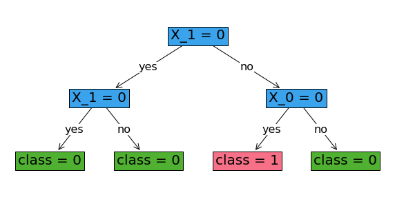
As we can see, with depth 2, we can achieve 100% in-sample accuracy.
[16]:
fig, ax = plt.subplots(figsize=(10, 5))
stcl.plot_tree(ax=ax, fontsize=20)
plt.show()
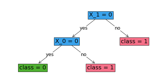
Tree with depth=2 and Positive _lambda
As we saw in the above example, with depth 2, we can fully classify the training data. However if we add a regularization term with a high enough value of _lambda, we can justify pruning one of the branching nodes to get a sparser tree. In the following, we observe that as we increase _lambda from 0 to 0.51, one of the branching nodes gets pruned and as a result, the in-sample accuracy drops to 92%.
[17]:
stcl = FlowOCT(solver="gurobi", depth=2, _lambda=0.51)
stcl.fit(X, y)
Set parameter Username
Academic license - for non-commercial use only - expires 2025-06-28
Set parameter TimeLimit to value 60
Set parameter NodeLimit to value 1073741824
Set parameter SolutionLimit to value 1073741824
Set parameter IntFeasTol to value 1e-06
Set parameter Method to value 3
Gurobi Optimizer version 10.0.2 build v10.0.2rc0 (mac64[arm])

CPU model: Apple M1 Pro
Thread count: 8 physical cores, 8 logical processors, using up to 8 threads

Optimize a model with 274 rows, 209 columns and 642 nonzeros
Model fingerprint: 0x3e3f455b
Variable types: 196 continuous, 13 integer (13 binary)
Coefficient statistics:
  Matrix range     [1e+00, 1e+00]
  Objective range  [5e-01, 5e-01]
  Bounds range     [1e+00, 1e+00]
  RHS range        [1e+00, 1e+00]
Found heuristic solution: objective -0.0000000
Presolve removed 250 rows and 187 columns
Presolve time: 0.00s
Presolved: 24 rows, 22 columns, 76 nonzeros
Found heuristic solution: objective 3.9200000
Variable types: 16 continuous, 6 integer (6 binary)

Root relaxation: objective 5.105000e+00, 14 iterations, 0.00 seconds (0.00 work units)

    Nodes    |    Current Node    |     Objective Bounds      |     Work
 Expl Unexpl |  Obj  Depth IntInf | Incumbent    BestBd   Gap | It/Node Time

     0     0    5.10500    0    2    3.92000    5.10500  30.2%     -    0s
H    0     0                       4.8600000    5.10500  5.04%     -    0s

Explored 1 nodes (14 simplex iterations) in 0.00 seconds (0.00 work units)
Thread count was 8 (of 8 available processors)

Solution count 3: 4.86 3.92 -0

Optimal solution found (tolerance 1.00e-04)
Best objective 4.860000000000e+00, best bound 4.860000000000e+00, gap 0.0000%
[17]:
FlowOCT(solver=gurobi,depth=2,time_limit=60,num_threads=None,verbose=False)
[18]:
predictions = stcl.predict(X)
print(f"In-sample accuracy is {np.sum(predictions==y)/y.shape[0]}")
In-sample accuracy is 0.9230769230769231
[19]:
fig, ax = plt.subplots(figsize=(10, 5))
stcl.plot_tree(ax=ax, fontsize=20)
plt.show()
Example 2: Different Objective Functions
In the following, we have a toy example with an imbalanced data, with the positive class being the minority class.
[20]:
'''
    X2
    |               |
    |               |
    1    + - -      |    -
    |               |
    |---------------|--------------
    |               |
    0    - - - +    |    - - -
    |    - - - -    |
    |______0________|_______1_______X1
'''
X = np.array([[0,0],[0,0],[0,0],[0,0],[0,0],[0,0],[0,0],[0,0],
              [1,0],[1,0],[1,0],
              [1,1],
              [0,1],[0,1],[0,1]])
y = np.array([0,0,0,0,0,0,0,1,
              0,0,0,
              0,
              1,0,0])
Tree with classification accuracy objective
[21]:
stcl_acc = FlowOCT(solver="gurobi", depth=2, obj_mode="acc")
stcl_acc.fit(X, y)
Set parameter Username
Academic license - for non-commercial use only - expires 2025-06-28
Set parameter TimeLimit to value 60
Set parameter NodeLimit to value 1073741824
Set parameter SolutionLimit to value 1073741824
Set parameter IntFeasTol to value 1e-06
Set parameter Method to value 3
Gurobi Optimizer version 10.0.2 build v10.0.2rc0 (mac64[arm])

CPU model: Apple M1 Pro
Thread count: 8 physical cores, 8 logical processors, using up to 8 threads

Optimize a model with 314 rows, 237 columns and 734 nonzeros
Model fingerprint: 0xa5b9a46b
Variable types: 224 continuous, 13 integer (13 binary)
Coefficient statistics:
  Matrix range     [1e+00, 1e+00]
  Objective range  [1e+00, 1e+00]
  Bounds range     [1e+00, 1e+00]
  RHS range        [1e+00, 1e+00]
Found heuristic solution: objective -0.0000000
Presolve removed 269 rows and 203 columns
Presolve time: 0.00s
Presolved: 45 rows, 34 columns, 134 nonzeros
Found heuristic solution: objective 13.0000000
Variable types: 27 continuous, 7 integer (7 binary)

Root relaxation: objective 1.400000e+01, 32 iterations, 0.00 seconds (0.00 work units)

    Nodes    |    Current Node    |     Objective Bounds      |     Work
 Expl Unexpl |  Obj  Depth IntInf | Incumbent    BestBd   Gap | It/Node Time

     0     0   14.00000    0    1   13.00000   14.00000  7.69%     -    0s

Cutting planes:
  MIR: 1
  Flow cover: 1

Explored 1 nodes (32 simplex iterations) in 0.00 seconds (0.00 work units)
Thread count was 8 (of 8 available processors)

Solution count 2: 13 -0

Optimal solution found (tolerance 1.00e-04)
Best objective 1.300000000000e+01, best bound 1.300000000000e+01, gap 0.0000%
[21]:
FlowOCT(solver=gurobi,depth=2,time_limit=60,num_threads=None,verbose=False)
[22]:
predictions = stcl_acc.predict(X)
print(f"In-sample accuracy is {np.sum(predictions==y)/y.shape[0]}")
In-sample accuracy is 0.8666666666666667
[23]:
stcl_acc.print_tree()
#########node  1
leaf 0
#########node  2
pruned
#########node  3
pruned
#########node  4
pruned
#########node  5
pruned
#########node  6
pruned
#########node  7
pruned
[24]:
fig, ax = plt.subplots(figsize=(10, 5))
stcl_acc.plot_tree(ax=ax, fontsize=20)
plt.show()
Tree with Balanced Classification Accuracy Objective
[25]:
stcl_balance = FlowOCT(
    solver="gurobi",
    depth=2,
    obj_mode="balance",
    _lambda=0,
    verbose=False,
)
stcl_balance.fit(X, y)
predictions = stcl_balance.predict(X)
print(f"In-sample accuracy is {np.sum(predictions==y)/y.shape[0]}")
Set parameter Username
Academic license - for non-commercial use only - expires 2025-06-28
Set parameter TimeLimit to value 60
Set parameter NodeLimit to value 1073741824
Set parameter SolutionLimit to value 1073741824
Set parameter IntFeasTol to value 1e-06
Set parameter Method to value 3
Gurobi Optimizer version 10.0.2 build v10.0.2rc0 (mac64[arm])

CPU model: Apple M1 Pro
Thread count: 8 physical cores, 8 logical processors, using up to 8 threads

Optimize a model with 314 rows, 237 columns and 734 nonzeros
Model fingerprint: 0x3bc6df12
Variable types: 224 continuous, 13 integer (13 binary)
Coefficient statistics:
  Matrix range     [1e+00, 1e+00]
  Objective range  [4e-02, 2e-01]
  Bounds range     [1e+00, 1e+00]
  RHS range        [1e+00, 1e+00]
Found heuristic solution: objective -0.0000000
Presolve removed 269 rows and 203 columns
Presolve time: 0.01s
Presolved: 45 rows, 34 columns, 134 nonzeros
Found heuristic solution: objective 0.5000000
Variable types: 27 continuous, 7 integer (7 binary)

Root relaxation: objective 7.500000e-01, 31 iterations, 0.00 seconds (0.00 work units)

    Nodes    |    Current Node    |     Objective Bounds      |     Work
 Expl Unexpl |  Obj  Depth IntInf | Incumbent    BestBd   Gap | It/Node Time

     0     0    0.75000    0    1    0.50000    0.75000  50.0%     -    0s
H    0     0                       0.5288462    0.75000  41.8%     -    0s
H    0     0                       0.6730769    0.75000  11.4%     -    0s
     0     0    0.67308    0    4    0.67308    0.67308  0.00%     -    0s

Cutting planes:
  MIR: 1
  Flow cover: 1

Explored 1 nodes (36 simplex iterations) in 0.01 seconds (0.00 work units)
Thread count was 8 (of 8 available processors)

Solution count 3: 0.673077 0.5 -0
No other solutions better than 0.673077

Optimal solution found (tolerance 1.00e-04)
Best objective 6.730769230769e-01, best bound 6.730769230769e-01, gap 0.0000%
In-sample accuracy is 0.8
[26]:
fig, ax = plt.subplots(figsize=(10, 5))
stcl_balance.plot_tree(ax=ax, fontsize=20)
plt.show()
As we can see, when we maximize accuracy, i.e., when obj_mode = 'acc', the optimal tree is just a single node without branching, predicting the majority class for the whole dataset. But when we change the objective mode to balanced accuracy, we account for the minority class by sacrificing the overal accuracy.
Example 3: UCI Data Example
In this section, we fit a tree of depth 3 on a real world dataset called the `balance dataset <https://archive.ics.uci.edu/ml/datasets/Balance+Scale>`__ from the UCI Machine Learning repository.
[27]:
import pandas as pd
from sklearn.model_selection import train_test_split
from odtlearn.datasets import balance_scale_data
[28]:
# read data
data = balance_scale_data()
print(f"shape{data.shape}")
data.columns
shape(625, 21)
[28]:
Index(['V2.1', 'V2.2', 'V2.3', 'V2.4', 'V2.5', 'V3.1', 'V3.2', 'V3.3', 'V3.4',
       'V3.5', 'V4.1', 'V4.2', 'V4.3', 'V4.4', 'V4.5', 'V5.1', 'V5.2', 'V5.3',
       'V5.4', 'V5.5', 'target'],
      dtype='object')
[29]:
y = data.pop("target")

X_train, X_test, y_train, y_test = train_test_split(
    data, y, test_size=0.33, random_state=42
)
[30]:
stcl = BendersOCT(solver="gurobi", depth=3, time_limit=200, obj_mode="acc", verbose=True)

stcl.fit(X_train, y_train)
Set parameter Username
Academic license - for non-commercial use only - expires 2025-06-28
Set parameter TimeLimit to value 200
Set parameter NodeLimit to value 1073741824
Set parameter SolutionLimit to value 1073741824
Set parameter LazyConstraints to value 1
Set parameter IntFeasTol to value 1e-06
Set parameter Method to value 3
Gurobi Optimizer version 10.0.2 build v10.0.2rc0 (mac64[arm])

CPU model: Apple M1 Pro
Thread count: 8 physical cores, 8 logical processors, using up to 8 threads

Optimize a model with 30 rows, 618 columns and 249 nonzeros
Model fingerprint: 0xaeff5467
Variable types: 463 continuous, 155 integer (155 binary)
Coefficient statistics:
  Matrix range     [1e+00, 1e+00]
  Objective range  [1e+00, 1e+00]
  Bounds range     [1e+00, 1e+00]
  RHS range        [1e+00, 1e+00]
Presolve removed 8 rows and 8 columns
Presolve time: 0.00s
Presolved: 22 rows, 610 columns, 233 nonzeros
Variable types: 463 continuous, 147 integer (147 binary)
Root relaxation presolved: 412 rows, 610 columns, 7100 nonzeros

Concurrent LP optimizer: primal simplex, dual simplex, and barrier
Showing barrier log only...

Root barrier log...

Ordering time: 0.00s

Barrier performed 0 iterations in 0.18 seconds (0.00 work units)
Barrier solve interrupted - model solved by another algorithm


Solved with dual simplex

Root relaxation: objective 4.180000e+02, 77 iterations, 0.01 seconds (0.00 work units)

    Nodes    |    Current Node    |     Objective Bounds      |     Work
 Expl Unexpl |  Obj  Depth IntInf | Incumbent    BestBd   Gap | It/Node Time

     0     0  418.00000    0    4          -  418.00000      -     -    0s
H    0     0                     269.0000000  418.00000  55.4%     -    0s
     0     0  418.00000    0    4  269.00000  418.00000  55.4%     -    0s
     0     2  413.60000    0    9  269.00000  413.60000  53.8%     -    0s
H  308   294                     272.0000000  413.60000  52.1%  75.5    1s
H  483   460                     274.0000000  413.60000  50.9%  75.6    1s
*  533   475              54     290.0000000  413.60000  42.6%  73.6    1s
  1143   887     cutoff   64       290.00000  412.40000  42.2%  78.6    5s
H 1310   970                     291.0000000  412.40000  41.7%  75.5    5s
  1556  1132  316.00000   35   26  291.00000  409.65561  40.8%  70.5   10s
  1629  1180  371.73684   22   25  291.00000  403.03327  38.5%  67.3   15s
  1797  1290  367.57918   36   10  291.00000  402.21668  38.2%  92.8   20s
H 2163  1398                     293.0000000  400.54472  36.7%  92.9   21s
* 2375  1361             111     296.0000000  399.64465  35.0%  91.6   22s
H 3419  1561                     299.0000000  398.14472  33.2%  86.5   24s
  3861  1733  358.57143   67   20  299.00000  398.14472  33.2%  87.2   25s
H 4454  1024                     312.0000000  398.14472  27.6%  85.7   25s
  8785  2721     cutoff   62       312.00000  358.67679  15.0%  82.5   30s
 16715  6109  313.50000   67   16  312.00000  338.60887  8.53%  69.7   35s
H17827  5595                     314.0000000  338.16497  7.70%  67.8   35s
 26793  9027  315.00000   77    8  314.00000  330.38947  5.22%  59.2   40s
H31789  9084                     315.0000000  329.54167  4.62%  57.5   43s
 33926  9710  318.00000   71    8  315.00000  328.75000  4.37%  56.7   45s
H35037  8771                     316.0000000  328.02174  3.80%  56.5   45s
H36500  6760                     318.0000000  327.50000  2.99%  56.0   46s
 42743  6716  322.50000   59   12  318.00000  325.00000  2.20%  54.1   50s
 54532  4635     cutoff   48       318.00000  321.00000  0.94%  50.5   55s
 65931  1611     cutoff   74       318.00000  319.48148  0.47%  47.7   60s

Cutting planes:
  MIR: 120
  Flow cover: 193
  Lazy constraints: 236

Explored 70775 nodes (3292092 simplex iterations) in 61.92 seconds (141.79 work units)
Thread count was 8 (of 8 available processors)

Solution count 10: 318 316 315 ... 290

Optimal solution found (tolerance 1.00e-04)
Best objective 3.180000000000e+02, best bound 3.180000000000e+02, gap 0.0000%

User-callback calls 150674, time in user-callback 1.85 sec
[30]:
BendersOCT(solver=gurobi,depth=3,time_limit=200,num_threads=None,verbose=True)
[31]:
stcl.print_tree()
#########node  1
branch on V3.2
#########node  2
branch on V3.1
#########node  3
branch on V5.1
#########node  4
branch on V2.1
#########node  5
branch on V5.1
#########node  6
branch on V4.1
#########node  7
branch on V2.1
#########node  8
leaf 2
#########node  9
leaf 3
#########node  10
leaf 3
#########node  11
leaf 2
#########node  12
leaf 3
#########node  13
leaf 2
#########node  14
leaf 2
#########node  15
leaf 3
[32]:
fig, ax = plt.subplots(figsize=(20, 10))
stcl.plot_tree(ax=ax, fontsize=20, color_dict={"node": None, "leaves": []})
plt.show()
[33]:
test_pred = stcl.predict(X_test)
print('The out-of-sample accuracy is {}'.format(np.sum(test_pred==y_test)/y_test.shape[0]))
The out-of-sample accuracy is 0.6859903381642513
Example 4: User-defined Weights
In this example, we’ll demonstrate how to use user-defined weights with FlowOCT and BendersOCT. We’ll use a small binary classification dataset and show how user-defined weights can affect the learned tree.
First, let’s create our small binary classification dataset:
[34]:
np.random.seed(42)
X = np.random.randint(0, 2, size=(20, 5))
y = np.random.randint(0, 2, size=20)

print("Dataset shape:", X.shape)
print("Class distribution:", np.bincount(y))
Dataset shape: (20, 5)
Class distribution: [ 6 14]
Now, let’s create weights that heavily favor class 1:
[35]:
weights = np.ones_like(y)
weights[y == 1] = 10

print("Weight distribution:")
print("Class 0:", weights[y == 0].mean())
print("Class 1:", weights[y == 1].mean())
Weight distribution:
Class 0: 1.0
Class 1: 10.0
FlowOCT with User-defined Weights
Let’s fit a FlowOCT model with user-defined weights and compare it to a model without the accuracy objective:
[36]:
# FlowOCT without custom weights
flow_oct_default = FlowOCT(solver="gurobi", obj_mode="acc", depth=2, time_limit=10)
flow_oct_default.fit(X, y)

# FlowOCT with custom weights
flow_oct_custom = FlowOCT(solver="gurobi", obj_mode="weighted", depth=2, time_limit=10)
flow_oct_custom.fit(X, y, weights=weights)

print("Default FlowOCT predictions:", flow_oct_default.predict(X))
print("User-defined weights FlowOCT predictions:", flow_oct_custom.predict(X))

print("Default FlowOCT accuracy:", (flow_oct_default.predict(X) == y).mean())
print("User-defined weights FlowOCT accuracy:", (flow_oct_custom.predict(X) == y).mean())
print("User-defined weights FlowOCT weighted accuracy:", np.average(flow_oct_custom.predict(X) == y, weights=weights))
Set parameter Username
Academic license - for non-commercial use only - expires 2025-06-28
Set parameter TimeLimit to value 10
Set parameter NodeLimit to value 1073741824
Set parameter SolutionLimit to value 1073741824
Set parameter IntFeasTol to value 1e-06
Set parameter Method to value 3
Gurobi Optimizer version 10.0.2 build v10.0.2rc0 (mac64[arm])

CPU model: Apple M1 Pro
Thread count: 8 physical cores, 8 logical processors, using up to 8 threads

Optimize a model with 414 rows, 316 columns and 1153 nonzeros
Model fingerprint: 0x1ad65f5a
Variable types: 294 continuous, 22 integer (22 binary)
Coefficient statistics:
  Matrix range     [1e+00, 1e+00]
  Objective range  [1e+00, 1e+00]
  Bounds range     [1e+00, 1e+00]
  RHS range        [1e+00, 1e+00]
Found heuristic solution: objective -0.0000000
Presolve removed 205 rows and 186 columns
Presolve time: 0.00s
Presolved: 209 rows, 130 columns, 660 nonzeros
Found heuristic solution: objective 14.0000000
Variable types: 112 continuous, 18 integer (18 binary)

Root relaxation: objective 1.966667e+01, 166 iterations, 0.00 seconds (0.00 work units)

    Nodes    |    Current Node    |     Objective Bounds      |     Work
 Expl Unexpl |  Obj  Depth IntInf | Incumbent    BestBd   Gap | It/Node Time

     0     0   19.66667    0    7   14.00000   19.66667  40.5%     -    0s
H    0     0                      16.0000000   19.66667  22.9%     -    0s
H    0     0                      17.0000000   19.00000  11.8%     -    0s
     0     0   18.50000    0    9   17.00000   18.50000  8.82%     -    0s

Cutting planes:
  Gomory: 13
  MIR: 6
  RLT: 20

Explored 1 nodes (198 simplex iterations) in 0.01 seconds (0.01 work units)
Thread count was 8 (of 8 available processors)

Solution count 4: 17 16 14 -0

Optimal solution found (tolerance 1.00e-04)
Best objective 1.700000000000e+01, best bound 1.700000000000e+01, gap 0.0000%
Set parameter Username
Academic license - for non-commercial use only - expires 2025-06-28
Set parameter TimeLimit to value 10
Set parameter NodeLimit to value 1073741824
Set parameter SolutionLimit to value 1073741824
Set parameter IntFeasTol to value 1e-06
Set parameter Method to value 3
Gurobi Optimizer version 10.0.2 build v10.0.2rc0 (mac64[arm])

CPU model: Apple M1 Pro
Thread count: 8 physical cores, 8 logical processors, using up to 8 threads

Optimize a model with 414 rows, 316 columns and 1153 nonzeros
Model fingerprint: 0xf6c20781
Variable types: 294 continuous, 22 integer (22 binary)
Coefficient statistics:
  Matrix range     [1e+00, 1e+00]
  Objective range  [1e+00, 1e+01]
  Bounds range     [1e+00, 1e+00]
  RHS range        [1e+00, 1e+00]
Found heuristic solution: objective -0.0000000
Presolve removed 205 rows and 186 columns
Presolve time: 0.00s
Presolved: 209 rows, 130 columns, 660 nonzeros
Found heuristic solution: objective 140.0000000
Variable types: 112 continuous, 18 integer (18 binary)

Root relaxation: objective 1.456667e+02, 173 iterations, 0.00 seconds (0.00 work units)

    Nodes    |    Current Node    |     Objective Bounds      |     Work
 Expl Unexpl |  Obj  Depth IntInf | Incumbent    BestBd   Gap | It/Node Time

     0     0  145.66667    0    7  140.00000  145.66667  4.05%     -    0s
H    0     0                     143.0000000  144.66667  1.17%     -    0s
     0     0  144.00000    0   11  143.00000  144.00000  0.70%     -    0s
     0     0  143.00000    0    6  143.00000  143.00000  0.00%     -    0s

Cutting planes:
  Gomory: 1
  MIR: 1
  RLT: 7

Explored 1 nodes (233 simplex iterations) in 0.01 seconds (0.01 work units)
Thread count was 8 (of 8 available processors)

Solution count 3: 143 140 -0

Optimal solution found (tolerance 1.00e-04)
Best objective 1.430000000000e+02, best bound 1.430000000000e+02, gap 0.0000%
Default FlowOCT predictions: [1 1 1 1 1 1 1 1 1 1 1 0 1 1 0 1 1 1 1 0]
Custom weights FlowOCT predictions: [1 1 1 1 1 1 1 1 1 1 1 0 1 1 0 1 1 1 1 0]

Default FlowOCT accuracy: 0.85
Custom weights FlowOCT accuracy: 0.85
Custom weights FlowOCT weighted accuracy: 0.9794520547945206
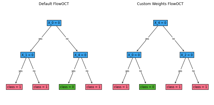
Let’s visualize both trees:
[37]:
fig, (ax1, ax2) = plt.subplots(1, 2, figsize=(10, 5))

flow_oct_default.plot_tree(ax=ax1, fontsize=10)
ax1.set_title("Default FlowOCT")

flow_oct_custom.plot_tree(ax=ax2, fontsize=10)
ax2.set_title("User-defined Weights FlowOCT")

plt.tight_layout()
plt.show()
BendersOCT with User-defined Weights
Now let’s do the same with BendersOCT:
[38]:
# BendersOCT without custom weights
benders_oct_default = BendersOCT(solver="gurobi", obj_mode="acc", depth=2, time_limit=10)
benders_oct_default.fit(X, y)

# BendersOCT with custom weights
benders_oct_custom = BendersOCT(solver="gurobi", obj_mode="weighted", depth=2, time_limit=10, verbose=False)
benders_oct_custom.fit(X, y, weights=weights)

print("Default BendersOCT predictions:", benders_oct_default.predict(X))
print("User-defined weights BendersOCT predictions:", benders_oct_custom.predict(X))

print("Default BendersOCT accuracy:", (benders_oct_default.predict(X) == y).mean())
print("User-defined weights BendersOCT accuracy:", (benders_oct_custom.predict(X) == y).mean())
print("User-defined weights BendersOCT weighted accuracy:", np.average(benders_oct_custom.predict(X) == y, weights=weights))
Set parameter Username
Academic license - for non-commercial use only - expires 2025-06-28
Set parameter TimeLimit to value 10
Set parameter NodeLimit to value 1073741824
Set parameter SolutionLimit to value 1073741824
Set parameter LazyConstraints to value 1
Set parameter IntFeasTol to value 1e-06
Set parameter Method to value 3
Gurobi Optimizer version 10.0.2 build v10.0.2rc0 (mac64[arm])

CPU model: Apple M1 Pro
Thread count: 8 physical cores, 8 logical processors, using up to 8 threads

Optimize a model with 14 rows, 56 columns and 53 nonzeros
Model fingerprint: 0x28902962
Variable types: 34 continuous, 22 integer (22 binary)
Coefficient statistics:
  Matrix range     [1e+00, 1e+00]
  Objective range  [1e+00, 1e+00]
  Bounds range     [1e+00, 1e+00]
  RHS range        [1e+00, 1e+00]
Presolve removed 4 rows and 4 columns
Presolve time: 0.00s
Presolved: 10 rows, 52 columns, 45 nonzeros
Variable types: 34 continuous, 18 integer (18 binary)
Root relaxation presolved: 22 rows, 50 columns, 140 nonzeros


Root relaxation: objective 2.000000e+01, 2 iterations, 0.00 seconds (0.00 work units)

    Nodes    |    Current Node    |     Objective Bounds      |     Work
 Expl Unexpl |  Obj  Depth IntInf | Incumbent    BestBd   Gap | It/Node Time

     0     0   20.00000    0    -          -   20.00000      -     -    0s
     0     0   20.00000    0    -          -   20.00000      -     -    0s
     0     0   20.00000    0    -          -   20.00000      -     -    0s
     0     0   20.00000    0    7          -   20.00000      -     -    0s
H    0     0                      14.0000000   20.00000  42.9%     -    0s
H    0     0                      16.0000000   20.00000  25.0%     -    0s
     0     0   19.50000    0    2   16.00000   19.50000  21.9%     -    0s
     0     0   19.26563    0    9   16.00000   19.26563  20.4%     -    0s
H    0     0                      17.0000000   19.26563  13.3%     -    0s
     0     0   19.00000    0    8   17.00000   19.00000  11.8%     -    0s
     0     0   18.96429    0    9   17.00000   18.96429  11.6%     -    0s
     0     0   18.95833    0    9   17.00000   18.95833  11.5%     -    0s
     0     0   18.85000    0    9   17.00000   18.85000  10.9%     -    0s
     0     0   18.85000    0    9   17.00000   18.85000  10.9%     -    0s
     0     0   18.76563    0   11   17.00000   18.76563  10.4%     -    0s
     0     0   18.74194    0   10   17.00000   18.74194  10.2%     -    0s
     0     0   18.73913    0    9   17.00000   18.73913  10.2%     -    0s
     0     0   18.59091    0    9   17.00000   18.59091  9.36%     -    0s
     0     0   18.50000    0    9   17.00000   18.50000  8.82%     -    0s
     0     0   18.50000    0    9   17.00000   18.50000  8.82%     -    0s
     0     0   18.37500    0    8   17.00000   18.37500  8.09%     -    0s
     0     0   18.33333    0    8   17.00000   18.33333  7.84%     -    0s
     0     0   18.33333    0    9   17.00000   18.33333  7.84%     -    0s
     0     0   18.31250    0    7   17.00000   18.31250  7.72%     -    0s
     0     0   18.30000    0    7   17.00000   18.30000  7.65%     -    0s
     0     0   18.16667    0    7   17.00000   18.16667  6.86%     -    0s
     0     0   18.14706    0    8   17.00000   18.14706  6.75%     -    0s
     0     0   18.09524    0   10   17.00000   18.09524  6.44%     -    0s
     0     0   18.07059    0   10   17.00000   18.07059  6.30%     -    0s
     0     0   18.03478    0   10   17.00000   18.03478  6.09%     -    0s
     0     0   18.01765    0   11   17.00000   18.01765  5.99%     -    0s
     0     0   18.01333    0   11   17.00000   18.01333  5.96%     -    0s
     0     0   18.00532    0   12   17.00000   18.00532  5.91%     -    0s
     0     0   18.00463    0   12   17.00000   18.00463  5.91%     -    0s
     0     0   17.95833    0    9   17.00000   17.95833  5.64%     -    0s
     0     0   17.91304    0    8   17.00000   17.91304  5.37%     -    0s
     0     0   17.91304    0    8   17.00000   17.91304  5.37%     -    0s
     0     0   17.90909    0    8   17.00000   17.90909  5.35%     -    0s
     0     0   17.90909    0   11   17.00000   17.90909  5.35%     -    0s
     0     0   17.89873    0   11   17.00000   17.89873  5.29%     -    0s
     0     0   17.89873    0   10   17.00000   17.89873  5.29%     -    0s
     0     2   17.89873    0   10   17.00000   17.89873  5.29%     -    0s

Cutting planes:
  Gomory: 1
  MIR: 11
  Flow cover: 5
  Lazy constraints: 46

Explored 16 nodes (312 simplex iterations) in 0.05 seconds (0.02 work units)
Thread count was 8 (of 8 available processors)

Solution count 3: 17 16 14

Optimal solution found (tolerance 1.00e-04)
Best objective 1.700000000000e+01, best bound 1.700000000000e+01, gap 0.0000%

User-callback calls 366, time in user-callback 0.02 sec
Set parameter Username
Academic license - for non-commercial use only - expires 2025-06-28
Set parameter TimeLimit to value 10
Set parameter NodeLimit to value 1073741824
Set parameter SolutionLimit to value 1073741824
Set parameter LazyConstraints to value 1
Set parameter IntFeasTol to value 1e-06
Set parameter Method to value 3
Gurobi Optimizer version 10.0.2 build v10.0.2rc0 (mac64[arm])

CPU model: Apple M1 Pro
Thread count: 8 physical cores, 8 logical processors, using up to 8 threads

Optimize a model with 14 rows, 56 columns and 53 nonzeros
Model fingerprint: 0x75b5cba0
Variable types: 34 continuous, 22 integer (22 binary)
Coefficient statistics:
  Matrix range     [1e+00, 1e+00]
  Objective range  [1e+00, 1e+01]
  Bounds range     [1e+00, 1e+00]
  RHS range        [1e+00, 1e+00]
Presolve removed 4 rows and 4 columns
Presolve time: 0.00s
Presolved: 10 rows, 52 columns, 45 nonzeros
Variable types: 34 continuous, 18 integer (18 binary)
Root relaxation presolved: 22 rows, 50 columns, 140 nonzeros


Root relaxation: objective 1.460000e+02, 2 iterations, 0.00 seconds (0.00 work units)

    Nodes    |    Current Node    |     Objective Bounds      |     Work
 Expl Unexpl |  Obj  Depth IntInf | Incumbent    BestBd   Gap | It/Node Time

     0     0  146.00000    0    -          -  146.00000      -     -    0s
     0     0  146.00000    0    -          -  146.00000      -     -    0s
     0     0  146.00000    0    -          -  146.00000      -     -    0s
     0     0  146.00000    0    7          -  146.00000      -     -    0s
H    0     0                     140.0000000  146.00000  4.29%     -    0s
     0     0  145.50000    0    4  140.00000  145.50000  3.93%     -    0s
     0     0  145.37500    0    7  140.00000  145.37500  3.84%     -    0s
H    0     0                     143.0000000  145.37500  1.66%     -    0s
     0     0  144.88542    0   10  143.00000  144.88542  1.32%     -    0s
     0     0  144.88194    0   10  143.00000  144.88194  1.32%     -    0s
     0     0  144.33333    0    7  143.00000  144.33333  0.93%     -    0s
     0     0  144.30000    0    7  143.00000  144.30000  0.91%     -    0s
     0     0  144.16667    0    7  143.00000  144.16667  0.82%     -    0s
     0     0  144.12500    0    9  143.00000  144.12500  0.79%     -    0s
     0     0  144.12500    0    9  143.00000  144.12500  0.79%     -    0s
     0     0  144.08333    0   11  143.00000  144.08333  0.76%     -    0s
     0     0  144.08036    0   11  143.00000  144.08036  0.76%     -    0s
     0     0  144.08036    0   11  143.00000  144.08036  0.76%     -    0s
     0     0  144.02737    0   10  143.00000  144.02737  0.72%     -    0s
     0     0  144.02737    0   11  143.00000  144.02737  0.72%     -    0s
     0     0  144.02632    0   11  143.00000  144.02632  0.72%     -    0s
     0     0  144.02632    0   10  143.00000  144.02632  0.72%     -    0s
     0     2  144.02632    0    9  143.00000  144.02632  0.72%     -    0s

Cutting planes:
  Gomory: 1
  MIR: 3
  Flow cover: 9
  Lazy constraints: 47

Explored 14 nodes (157 simplex iterations) in 0.03 seconds (0.01 work units)
Thread count was 8 (of 8 available processors)

Solution count 2: 143 140

Optimal solution found (tolerance 1.00e-04)
Best objective 1.430000000000e+02, best bound 1.430000000000e+02, gap 0.0000%
Default BendersOCT predictions: [1 1 1 1 1 1 1 1 1 1 1 0 1 1 0 1 1 1 1 0]
Custom weights BendersOCT predictions: [1 1 1 1 1 1 1 1 1 1 1 0 1 1 0 1 1 1 1 0]

Default BendersOCT accuracy: 0.85
Custom weights BendersOCT accuracy: 0.85

User-callback calls 283, time in user-callback 0.01 sec
Custom weights BendersOCT weighted accuracy: 0.9794520547945206
[39]:
fig, (ax1, ax2) = plt.subplots(1, 2, figsize=(10, 5))

benders_oct_default.plot_tree(ax=ax1, fontsize=10)
ax1.set_title("Default BendersOCT")

benders_oct_custom.plot_tree(ax=ax2, fontsize=10)
ax2.set_title("User-defined Weights BendersOCT")

plt.tight_layout()
plt.show()
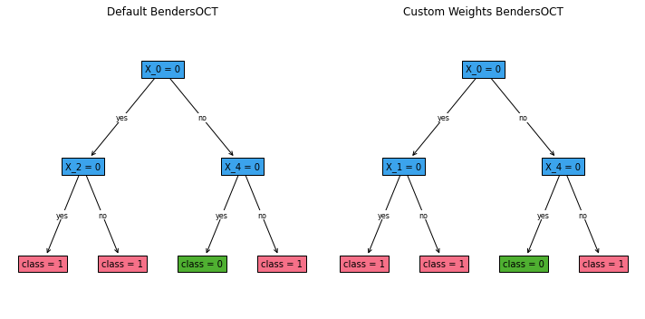
In this example, we’ve demonstrated how to use user-defined weights with both FlowOCT and BendersOCT. By setting obj_mode="weighted" and providing weights during the fit method call, we can influence the importance of different samples in the training process. The user-defined weights in this example heavily favor class 1, which may result in trees that are more likely to predict class 1, potentially at the cost of overall accuracy. However, this can be useful in scenarios where
misclassifying one class is more costly than misclassifying the other, or when dealing with imbalanced datasets. Note that the actual results may vary due to the random nature of the dataset and the optimization process. You may want to run the code multiple times or with different random seeds to get a better understanding of the effects of user-defined weights.
References
Dua, D. and Graff, C. (2019). UCI Machine Learning Repository. Irvine, CA: University of California, School of Information and Computer Science.
Aghaei, S., Gómez, A., & Vayanos, P. (2021). Strong optimal classification trees. arXiv preprint arXiv:2103.15965. https://arxiv.org/abs/2103.15965.